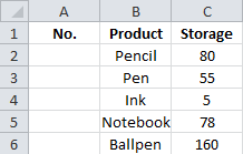
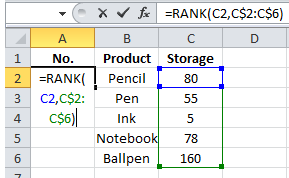
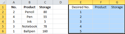
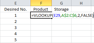
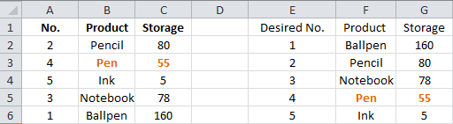
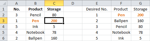
, trin 1: indsættelse af en ny kolonne i begyndelsen af originale data.,,,,, trin 2: følger vores eksempel, ind i formlen, = rang (c2, c 2: c 6 dollars), i celle a2 eller originale produkter ved oplagring, og tryk den ind, nøgle.,,,,, trin 3: udvælgelse og fremhæve den række a2: a6, og tryk, hjem, > >, fyld, > >,, at kopiere en formel til andre celler.,, trin 4: kopi af titlerne på de oprindelige data, og sæt dem desuden oprindelige tabel e1: g1, som f.eks.,, trin 4: i den ønskede - kolonne, indsættes følgenumre, den samme ordre.So in our example, enter 1, 2, … in the Desired No. column same as those in Column A. See the following screen shot:,,,,,Step 5: Enter the formula of ,,=VLOOKUP(E2,A$2:C$6,2,FALSE),, in the Cell F2, and press the ,Enter, key.,,,,,This formula will look for the value of Desired NO. in the original table, and show the corresponding product name in the cell.,,,Note,:,,(1) If repeats or ties happen in the Product column or Storage column, you’d better apply this function ,,=IFERROR(VLOOKUP(E2,A$2:C$6,2,FALSE), VLOOKUP(E2,A$2:C$6,2,TRUE)),,,,(2) If you are using Microsoft Excel 2003, both functions above are invalid, but you can use this one ,,=IF(ISERROR(VLOOKUP(E2,A$2:C$6,2,FALSE)), VLOOKUP(E2,A$2:C$6,2,TRUE), VLOOKUP(E2,A$2:C$6,2,FALSE)),,,, trin 6: angiv antal f2: g6, og tryk, hjem, > >, fyld, > >,,, og fyld, > >,,.,, så vil du få nye oplagrings - tabel sortering i ned for af lagre, jf. følgende skærm, hvis din stationære butik skød:,,,,, køb en anden 145 penne, og nu har du 200 penne i alt.bare ændre den oprindelige tab af pen er oplagring, vil du se den nye tabel er ajourført i et blink med øjnene, jf. følgende skærm skød:,,,,,,